A deep dive into Deepfakes

Posted by Nick Ashworth 2025-05-29

Deepfakes are a common topic in the AI community, but how do they actually work? In this post, we will explore the technology behind deepfakes, how they are created, and the methods used to detect them in real time.

What are Deepfakes?

Deepfakes are one of the most well-known and infamous examples of synthetic video generation, with numerous high-profile cases of their misuse. At their most basic, deepfakes are videos that have been manipulated to replace one person’s likeness with another’s. Over the years, they have evolved from only being able to edit pre-recorded videos to being able to generate real-time video streams. However, despite the bad reputation deepfakes have earned in the media, their origin is relatively benign. The models used to generate deepfakes are based on ones used by the animation industry for motion capture, which is one of the reasons why they are both so effective and so easy to use.

Unlike many other synthetic video generation models, deepfakes can be created with relatively little data, and run on almost any modern computer. This makes them accessible to a wide range of users, from hobbyists to professionals.

Creating Deepfakes

For this example, we will use the DeepFaceLab, an open-source tool for creating deepfakes. In our case, we will be using the 2D face replacement model, which is the most common type of deepfake. This is the technique most often referenced in the media, as it only requires a single image of the target face to create the deepfake. In our case, we will be using a single image of Vladimir Putin, but you can use any image you like.

Facial Landmark Detection

Our first step in this technique is to detect the facial features of the host face, in this case me. This is done using a facial landmark detection model, which identifies key points on the face such as the eyes, nose, and mouth. In our case, we’re using YOLOv5, a relatively older model.

Example of Facial Landmark Detection

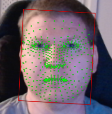An example of facial landmark detection within DeepFaceLive. Here the model has detected the key points on my face, which will be used to align the target face.

Face Alignment and Swapping

Once the facial landmarks have been detected, the next step is to align the target face with the host face. At its most basic level, this is done by rotating and scaling the target face, so that the key points from the landmark detection match the key points of the host face.

After the target face has been aligned, it is then swapped with the host face. This is done by replacing the pixels of the host face with the pixels of the target face, while preserving the facial landmarks. Most deepfake models will fill in the gaps in the target face with either a simple color fill or a more complex inpainting model, which will attempt to fill in the gaps with pixels that match the surrounding area. Depending upon the faces being swapped, this can lead ghosting artifacts, especially around the hairline.

Example of Face Alignment and Swapping

An example of the host face (me) that we will be using for the deepfake.

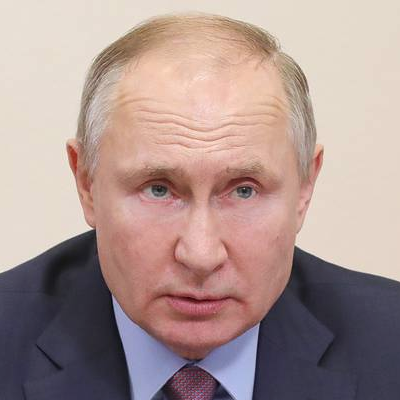An example of the target face (Vladimir Putin) that we will be using for the deepfake.

An example of the face swapping process, where the target face has been aligned and swapped with the host face.

And that’s it! We now have a deepfake video of me with Vladimir Putin’s face. You can use tools like OBS to stream the video in real-time, or you can save it as a video file.

Detecting Deepfakes

Now that we’ve shown how easy it is to create a deepfake, let’s take a look at how we can detect them in real-time. There are several methods for detecting deepfakes, but my personal favorite is using color histogram analysis. This method is based on the fact that deepfakes often have a different color distribution than real videos, due to the way they are generated.

Color Histogram Analysis

Histograms are a common tool in computer vision, and they are used to represent the distribution of pixel values in an image. They’re often used to compare images, and to correct for lighting conditions. In the case of deepfakes, we’ll be looking at the individual color channels (red, green, and blue) of the image, and seeing if they match the expected distribution of a real image.

For this example, we’ll be using OpenCV to calculate the histograms and Matplotlib to visualize the results. The code below will calculate the histograms for the red, green, and blue channels of the image, and then plot them.

import cv2 # OpenCV for image processing
import matplotlib.pyplot as plt # Matplotlib for plotting histograms

import tkinter as tk # Tkinter for GUI
from tkinter import filedialog # File dialog for selecting images

root = tk.Tk()
root.withdraw()

def show_image_histogram(image_path):
    # Load image
    img = cv2.imread(image_path)
    if img is None:
        raise FileNotFoundError("Image not found or invalid path.")

    # Check if image is grayscale or color
    if len(img.shape) == 2 or img.shape[2] == 1:
        # Grayscale image
        plt.figure()
        plt.title("Grayscale Histogram")
        plt.xlabel("Pixel Value")
        plt.ylabel("Frequency")
        hist = cv2.calcHist([img], [0], None, [256], [0, 256])
        plt.plot(hist, color='black')
        plt.xlim([0, 256])
        plt.show()
    else:
        # Color image: convert BGR to RGB for consistent plotting
        img_rgb = cv2.cvtColor(img, cv2.COLOR_BGR2RGB)
        colors = ('r', 'g', 'b')
        plt.figure()
        plt.title("Color Histogram")
        plt.xlabel("Pixel Value")
        plt.ylabel("Frequency")

        for i, color in enumerate(colors):
            hist = cv2.calcHist([img], [i], None, [256], [0, 256])
            plt.plot(hist, color=color)
            plt.xlim([0, 256])

        plt.show()

file_types = (
        ("Image files", "*.png *.jpg *.jpeg *.gif *.bmp"),
        ("All files", "*.*")
    )
file_path = filedialog.askopenfilename(title="Select an image for Histograms", filetypes=file_types)

if file_path:
    show_image_histogram(file_path)
else:
    print("No file selected.")

When we run this code on our images, we get the following histograms:

Example of Color Histogram Analysis

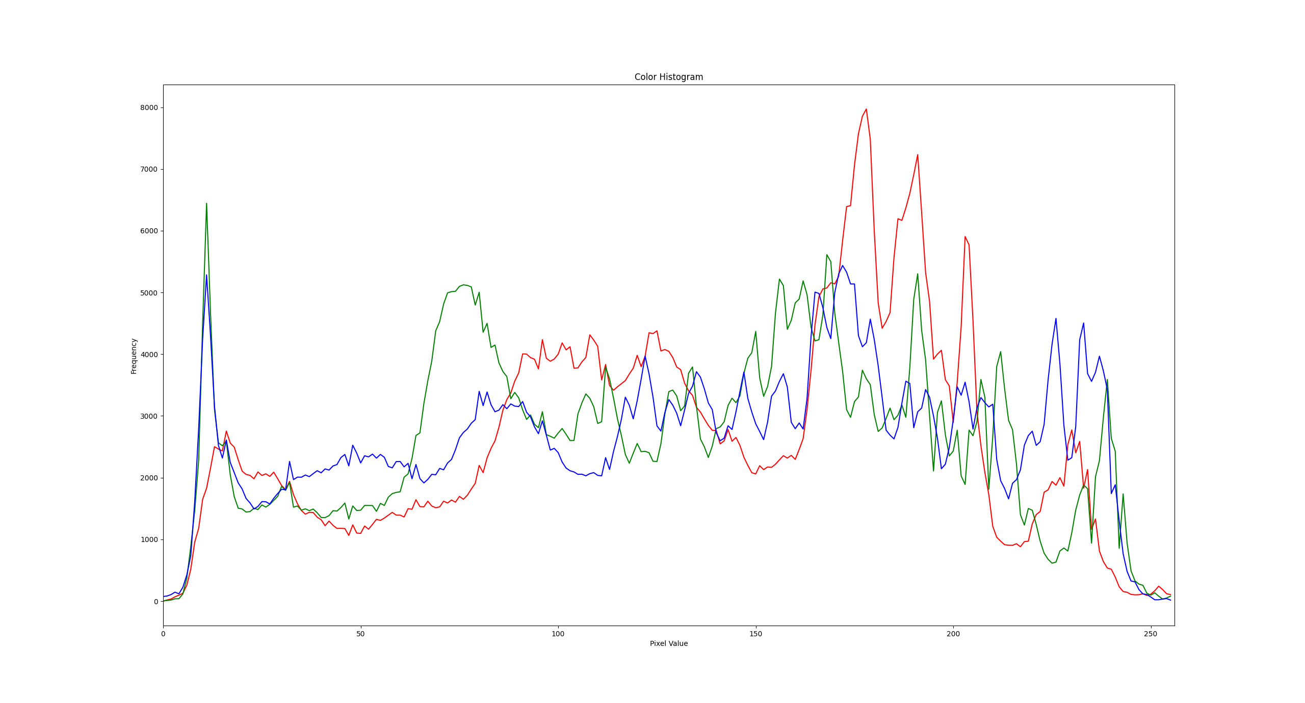An example of the color histogram for the host face (me). The red, green, and blue channels are shown in red, green, and blue respectively.

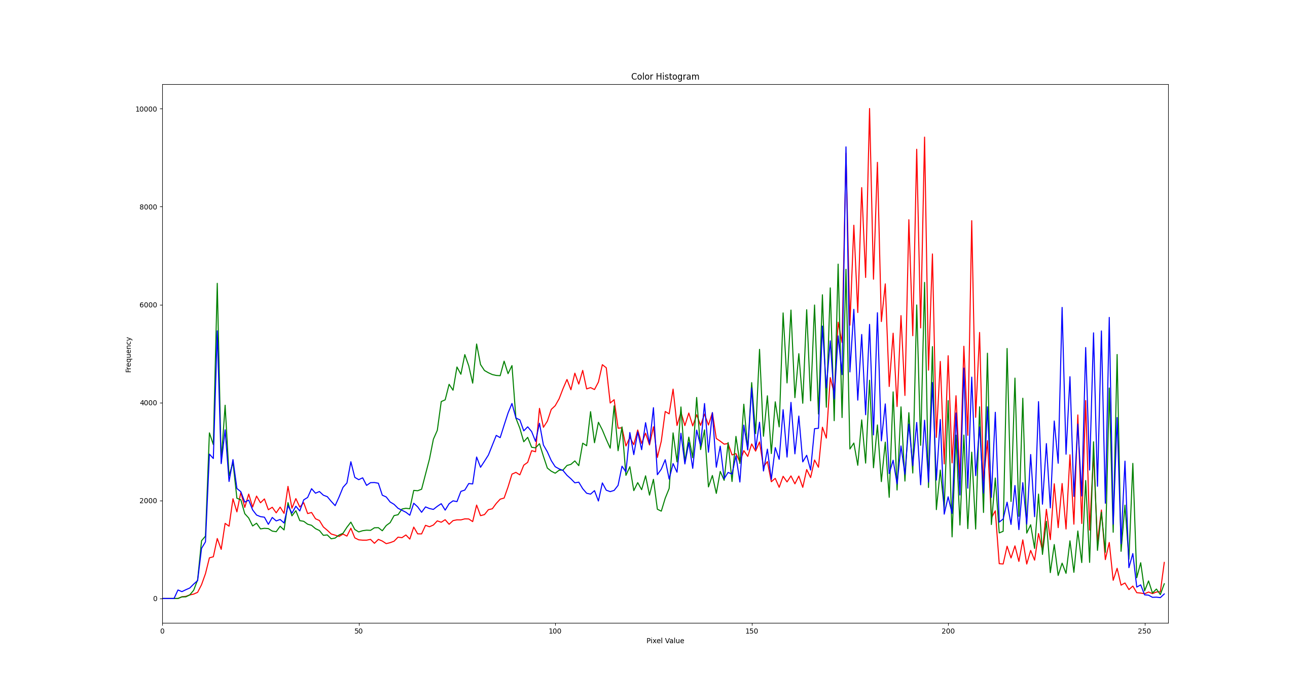An example of the color histogram for the deepfaked image. The red, green, and blue channels are shown in red, green, and blue respectively.

As you can see, the histogram for the deepfaked image is much noiser and jagged than the histogram for the host face. This is because the deepfake model has generated pixels that don’t match the expected distribution of a real image.

I personally like this method because it is simple to implement and can be done in real-time. It requires only a single image to calculate the expected distribution, and the code is easy to turn into a microservice. One of the big problems with deepfakes is how they quickly spread on social media, so techniques that are lightweight and can be run as microservices during the upload process are ideal.

However, this method is not foolproof, as it can be fooled by high-quality deepfakes that have been carefully crafted to match the expected distribution. It’s very much an 80% solution, but it is a good starting point for those who want to get into deepfake detection.

Conclusion

We hope you enjoyed this deep dive into deepfakes and how they are created and detected. We’ll be doing more with deepfakes later this year at DEFCON33, as an event we are calling “Deepfake Karaoke”. If you want to demonstrate your own deepfake detectors, or just want to see some funny deepfakes, come and join us!